Cook your First U-Net in PyTorch
A magic recipe to empower your image segmentation projects

U-Net is a deep learning architecture used for semantic segmentation tasks in image analysis. It was introduced by Olaf Ronneberger, Philipp Fischer, and Thomas Brox in a paper titled “U-Net: Convolutional Networks for Biomedical Image Segmentation”.
It is particularly effective for biomedical image segmentation tasks because it can handle images of arbitrary size and produces smooth, high-quality segmentation masks with sharp object boundaries. It has since been widely adopted in many other image segmentation tasks, such as in satellite and aerial imagery analysis, as well as in natural image segmentation.
In this tutorial, we will learn more about U-Net, how it works, and cook our own recipe -implementation- using PyTorch. So, let’s go!
How does it work?
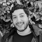
The U-Net architecture consists of two parts: an encoder and a decoder.

Encoder(Contraction Path)
The encoder is a series of convolutional and pooling layers that progressively downsample the input image to extract features at multiple scales.
In the Encoder, the size of the image is gradually reduced while the depth gradually increases. This basically means the network learns the “WHAT” information in the image, however, it has lost the “WHERE” information.
Decoder(Expansion Path)
The decoder consists of a series of convolutional and upsampling layers that upsample the feature maps to the original input image size while also incorporating the high-resolution features from the encoder. This allows the decoder to produce segmentation masks that have the same size as the original input image.
You can learn more about the upsampling and the transposed convolution from this great article.
In the Decoder, the size of the image gradually increases while the depth gradually decreases. This basically means the network learns the “WHERE” information in the image, by gradually applying up-sampling.
Final Layer
At the final layer, a 1x1 convolution is used to map each 64-component feature vector to the desired number of classes.
Our cooking recipe!
We will do a very straightforward implementation, it will be good to put the above image in front of you while coding.
Imports
First, the necessary modules are imported from the torch and torchvision packages, including the nn module for building neural networks and the pre-trained models provided in torchvision.models. The relu function is also imported from torch.nn.functional.
import torch
import torch.nn as nn
from torchvision import models
from torch.nn.functional import relu
UNet Class
Then, a custom class UNet is defined as a subclass of nn.Module. The __init__ method initializes the architecture of the U-Net by defining the layers for both the encoder and decoder parts of the network. The argument n_class specifies the number of classes for the segmentation task.
class UNet(nn.Module):
    def __init__(self, n_class):
        super().__init__()

        # Encoder
        # In the encoder, convolutional layers with the Conv2d function are used to extract features from the input image.
        # Each block in the encoder consists of two convolutional layers followed by a max-pooling layer, with the exception of the last block which does not include a max-pooling layer.
        # -------
        # input: 572x572x3
        self.e11 = nn.Conv2d(3, 64, kernel_size=3, padding=1) # output: 570x570x64
        self.e12 = nn.Conv2d(64, 64, kernel_size=3, padding=1) # output: 568x568x64
        self.pool1 = nn.MaxPool2d(kernel_size=2, stride=2) # output: 284x284x64

        # input: 284x284x64
        self.e21 = nn.Conv2d(64, 128, kernel_size=3, padding=1) # output: 282x282x128
        self.e22 = nn.Conv2d(128, 128, kernel_size=3, padding=1) # output: 280x280x128
        self.pool2 = nn.MaxPool2d(kernel_size=2, stride=2) # output: 140x140x128

        # input: 140x140x128
        self.e31 = nn.Conv2d(128, 256, kernel_size=3, padding=1) # output: 138x138x256
        self.e32 = nn.Conv2d(256, 256, kernel_size=3, padding=1) # output: 136x136x256
        self.pool3 = nn.MaxPool2d(kernel_size=2, stride=2) # output: 68x68x256

        # input: 68x68x256
        self.e41 = nn.Conv2d(256, 512, kernel_size=3, padding=1) # output: 66x66x512
        self.e42 = nn.Conv2d(512, 512, kernel_size=3, padding=1) # output: 64x64x512
        self.pool4 = nn.MaxPool2d(kernel_size=2, stride=2) # output: 32x32x512

        # input: 32x32x512
        self.e51 = nn.Conv2d(512, 1024, kernel_size=3, padding=1) # output: 30x30x1024
        self.e52 = nn.Conv2d(1024, 1024, kernel_size=3, padding=1) # output: 28x28x1024


        # Decoder
        self.upconv1 = nn.ConvTranspose2d(1024, 512, kernel_size=2, stride=2)
        self.d11 = nn.Conv2d(1024, 512, kernel_size=3, padding=1)
        self.d12 = nn.Conv2d(512, 512, kernel_size=3, padding=1)

        self.upconv2 = nn.ConvTranspose2d(512, 256, kernel_size=2, stride=2)
        self.d21 = nn.Conv2d(512, 256, kernel_size=3, padding=1)
        self.d22 = nn.Conv2d(256, 256, kernel_size=3, padding=1)

        self.upconv3 = nn.ConvTranspose2d(256, 128, kernel_size=2, stride=2)
        self.d31 = nn.Conv2d(256, 128, kernel_size=3, padding=1)
        self.d32 = nn.Conv2d(128, 128, kernel_size=3, padding=1)

        self.upconv4 = nn.ConvTranspose2d(128, 64, kernel_size=2, stride=2)
        self.d41 = nn.Conv2d(128, 64, kernel_size=3, padding=1)
        self.d42 = nn.Conv2d(64, 64, kernel_size=3, padding=1)

        # Output layer
        self.outconv = nn.Conv2d(64, n_class, kernel_size=1)
In the U-Net paper they used 0 padding and applied post-processing teachiques to restore the original size of the image, however here, we uses 1 padding so that final feature map is not cropped and to eliminate any need to apply post-processing to our output image.
Forward Method
The forward method specifies how the input is processed through the network. The input image is first passed through the encoder layers to extract the features. Then, the decoder layers are used to upsample the features to the original image size while concatenating the corresponding encoder feature maps. Finally, the output layer uses a 1x1 convolutional layer to map the features to the desired number of output classes.
    def forward(self, x):
        # Encoder
        xe11 = relu(self.e11(x))
        xe12 = relu(self.e12(xe11))
        xp1 = self.pool1(xe12)

        xe21 = relu(self.e21(xp1))
        xe22 = relu(self.e22(xe21))
        xp2 = self.pool2(xe22)

        xe31 = relu(self.e31(xp2))
        xe32 = relu(self.e32(xe31))
        xp3 = self.pool3(xe32)

        xe41 = relu(self.e41(xp3))
        xe42 = relu(self.e42(xe41))
        xp4 = self.pool4(xe42)

        xe51 = relu(self.e51(xp4))
        xe52 = relu(self.e52(xe51))

        # Decoder
        xu1 = self.upconv1(xe52)
        xu11 = torch.cat([xu1, xe42], dim=1)
        xd11 = relu(self.d11(xu11))
        xd12 = relu(self.d12(xd11))

        xu2 = self.upconv2(xd12)
        xu22 = torch.cat([xu2, xe32], dim=1)
        xd21 = relu(self.d21(xu22))
        xd22 = relu(self.d22(xd21))

        xu3 = self.upconv3(xd22)
        xu33 = torch.cat([xu3, xe22], dim=1)
        xd31 = relu(self.d31(xu33))
        xd32 = relu(self.d32(xd31))

        xu4 = self.upconv4(xd32)
        xu44 = torch.cat([xu4, xe12], dim=1)
        xd41 = relu(self.d41(xu44))
        xd42 = relu(self.d42(xd41))

        # Output layer
        out = self.outconv(xd42)

        return out
Don’t forget to hit the Clap and Follow buttons to help me write more articles like this.
That it is!
Congratulations on successfully implementing your first U-Net model in PyTorch! By following this recipe, you have gained the knowledge to implement U-Net and can now apply it to any image segmentation problem you may encounter in the future. However, verifying the sizes and channel numbers is important to ensure compatibility. The U-Net architecture is a powerful tool in your arsenal that can be applied to various tasks, including medical imaging and autonomous driving. So, go ahead and grab any image segmentation dataset from the internet and start testing your code!
For convenience, I have added a simple test script in this repository.
The script generates random images and masks and trains the U-net model to segment the images. It has a function called generate_random_data() that creates input images and their corresponding masks with geometric shapes like triangles, circles, squares, and crosses. The U-net model is trained using these random images and masks. The trained model is then tested on new random images and the segmentation results are plotted using the plot_img_array() function. The script uses PyTorch to train the U-net model and also uses various functions to add shapes to the input images and masks.
consider downloading it and running the tests using this snippet:
import test
test.run(UNet)
Final Thoughts
In conclusion, the U-Net architecture has become incredibly popular in the computer vision community due to its effectiveness in solving various image segmentation tasks. Its unique design, which includes a contracting path followed by an expanding path, allows it to capture both local and global features of an image while preserving spatial information.
Moreover, the flexibility of the U-Net architecture makes it possible to modify and improve the network to suit specific needs. Researchers have proposed various modifications to the original U-Net architecture, including changing the convolutional layers, incorporating attention mechanisms, and adding skip connections, among others. These modifications have resulted in improved performance and better segmentation results in various applications.
Overall, the U-Net architecture has proven to be a reliable and versatile solution for image segmentation tasks. As computer vision continues to advance, it’s likely that we’ll see further innovations and modifications to the U-Net architecture to improve its performance and make it even more effective in solving real-world problems.
Don’t hesitate to share your thoughts with me!